May 26, 2024 separationspython

McCabe-Thiele Method in Python

A step-by-step implementation of stage counting for binary distillation in Python

Introduction

This post gives a brief overview of the McCabe-Thiele method for binary distillation and a demonstration of how to implement it in Python. I’m making this primarily due to my experiences both as a student and TA for ChE 62 (Separation Processes) at Caltech; I was surprised to find that there are few resources available online that provide a clean, simple, step-by-step guide to implementing the McCabe-Thiele method in Python.

I’ll assume that readers are generally familiar with the McCabe-Thiele method. If you’re not, I recommend reading the Wikipedia page for the McCabe-Thiele method before proceeding. Alternatively, for much more detail, see the chapter entitled “Distillation of Binary Mixtures” in any edition of Separation Process Principles by Seader, Henley, and Roper.

Problem Statement

A continuous, steady-state distillation column with a total condenser and partial reboiler is separating 100 kmol/h of a 55 mol% methanol, 45 mol% water feed at 1 atm. We desire a distillate product that is 90 mol% methanol and a bottoms product that is 5 mol% methanol. Determine the plate on which the feed should be introduced and the total number of equilibrium stages required. Assume constant molar overflow.

Relevant Equations for the McCabe-Thiele Method

We’ll get the vapor-liquid equilibrium (VLE) data for the binary mixture from experimental data (we could also use an equation of state model to simulate the data, but that’s beyond the scope of this post). Next, the rectifying line and stripping line are constructed using the following equations since we are assuming constant molar overflow:

\begin{align} y &= \left(\frac{R}{R + 1}\right) x + \left(\frac{1}{R + 1}\right)x_D &\text{(rectifying)} \htmlId{eq:rectifyingline}{\tag{1}} \\ y &= \left(\frac{V_B + 1}{V_B}\right) x - \left(\frac{1}{V_B}\right)x_B &\text{(stripping)} \htmlId{eq:strippingline}{\tag{2}} \end{align}

where $x$ and $y$ are the mole fractions of the light component in the liquid and vapor phases, respectively; the reflux ratio $R=L/D$ ; the boilup ratio $V_B=\overline{V}/B$ ; $x_D$ ( $x_B$ ) and $y_D$ ( $y_B$ ) are the mole fractions of the light component in the distillate (bottoms); and $L$ , $V$ , $D$ , and $B$ are the liquid, vapor, distillate, and bottoms flow rates, respectively, where an overline represents that the flow rate is in the stripping section. Note: This notation is consistent with Separation Process Principles, 4e.

Python Implementation

We begin by loading in VLE data for methanol and water from the file methanol_water_vle_data.csv. This data was adapted from Vapor-Liquid Equilibrium Data Collection by J. Gmehling and U. Onken, 1977, Dechema, Frankfurt, Germany, vol. 1, p. 60. We’ll then plot the data to visualize the VLE curve and plot the 1:1 line ( $y$ = $x$ ) for reference. Additionally, we’ll plot the distillate, bottoms, and feed compositions on the plot.

# import necessary libraries
import numpy as np
import pandas as pd
from scipy.optimize import fsolve
import matplotlib.pyplot as plt
plt.style.use('ggplot')

# load data
data = pd.read_csv('methanol_water_vle_data.csv')
x_methanol = data['x_methanol']
y_methanol = data['y_methanol']

# set up plot
fig, ax = plt.subplots()
ax.plot(x_methanol, y_methanol, 'o-', color='blue', markersize=4)
ax.plot([0, 1], [0, 1], 'k')  # y = x

# constants for operating lines
R, x_D = 1.25, 0.90  # reflux ratio and distillate composition
B, x_B = 2.0, 0.05  # boilup ratio and bottoms composition
z = 0.55  # feed composition

# plot distillate, bottoms, and feed compositions
points = [x_D, x_B, z]
labels = [r'$x_D$', r'$x_B$', r'$z$']
for point, label in zip(points, labels):
    ax.plot([point, point], [0, point], color='k', linestyle='--')

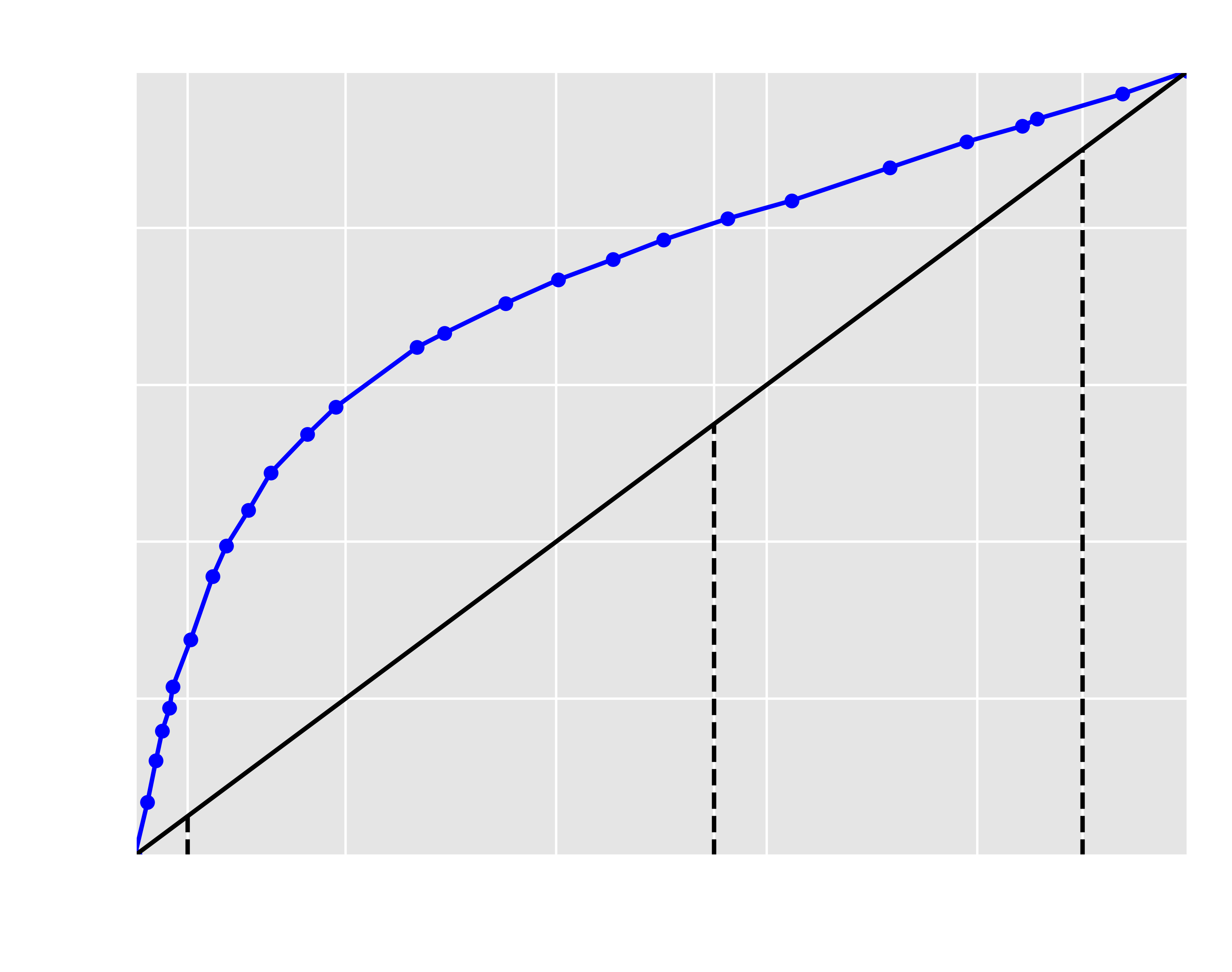
At this point, our plot should look like Figure 1 below. The VLE data is plotted in blue, the 1:1 line is in black, and the distillate, bottoms, and feed compositions are shown as dashed lines.

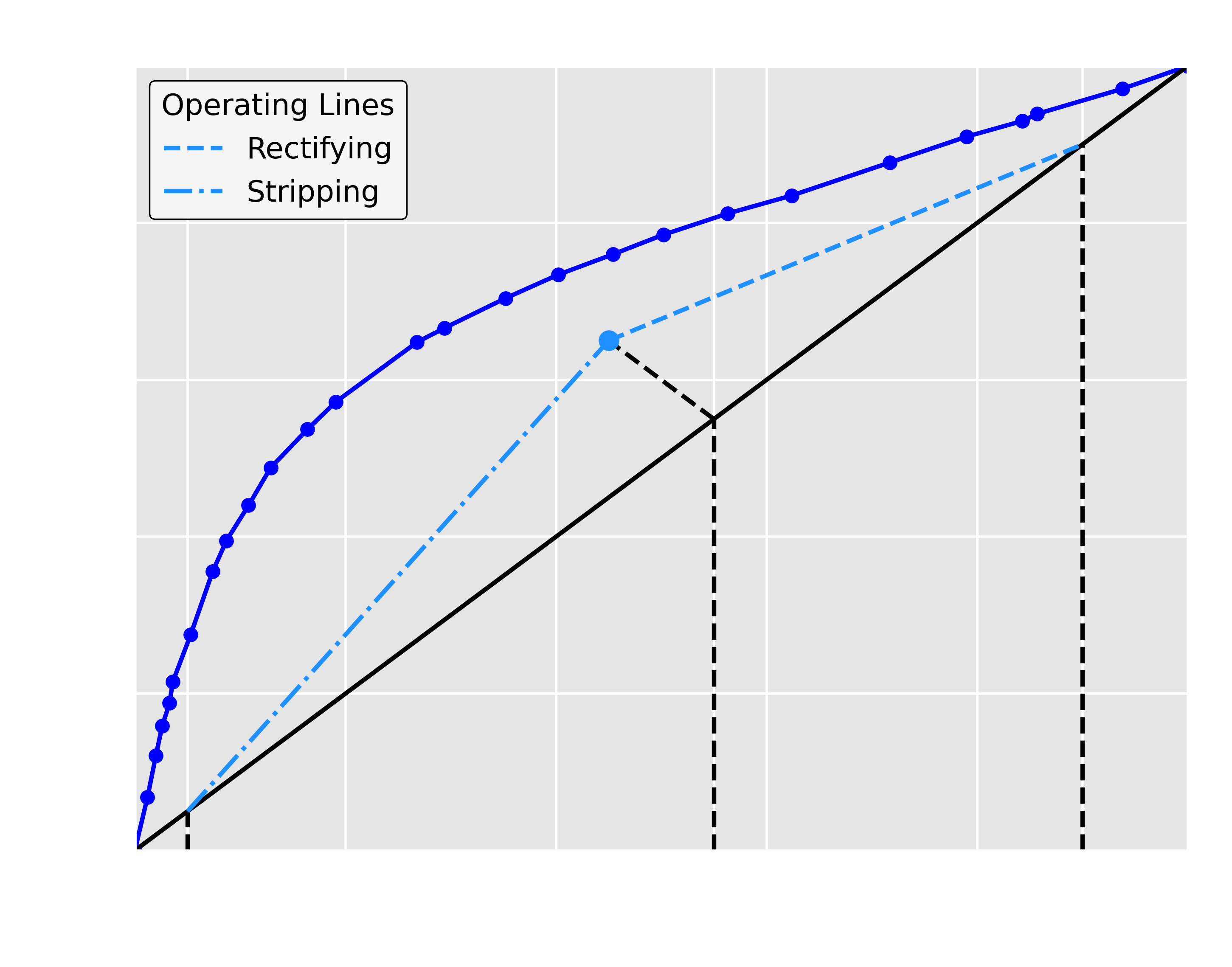
methanol water VLE data — Figure 1: Methanol-water VLE data with given stream compositions and 1:1 line.

Next, we can add our operating lines to the plot; luckily, we have all the information we need to directly use Equations $\href{#eq:rectifyingline}{(1)}$ and $\href{#eq:strippingline}{(2)}$ . We can find the intersection of the rectifying and stripping lines numerically using scipy.optimize.fsolve. This will allow us to create a cleaner plot by only plotting the rectifying and stripping lines up to the intersection point. Moreover, this will allow us to plot the q-line, as the q-line will pass through the intersection point and the 1:1 line.

# operating line functions
def top_line(x): return R / (R + 1) * x + x_D / (R + 1)
def bottom_line(x): return (B + 1) / B * x - x_B / B

# finding intersection of operating lines
intersection_x = fsolve(lambda x: top_line(x) - bottom_line(x), 0.5)[0]
intersection_y = top_line(intersection_x)
ax.plot(intersection_x, intersection_y, 'o', color='dodgerblue', zorder=10)

def plot_line_and_markers(x_range, function, color, label, ls='-'):
    x_vals = np.linspace(*x_range, 100)
    ax.plot(x_vals, function(x_vals), color=color, label=label, ls=ls)

# plot operating lines
plot_line_and_markers((intersection_x, x_D), top_line, 'dodgerblue', 'Rectifying', '--')
plot_line_and_markers((x_B, intersection_x), bottom_line, 'dodgerblue', 'Stripping', '-.')

# q-line
ax.plot([z, intersection_x], [z, intersection_y], 'k--')

The plot should now look like Figure 2 below.

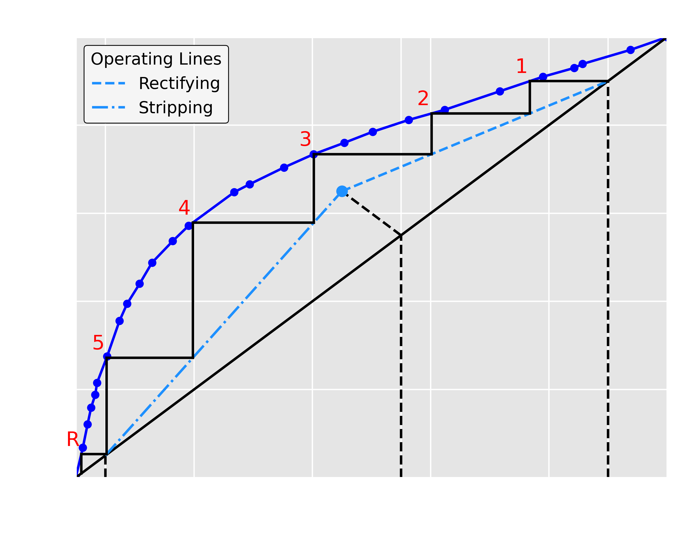
base of McCabe-Thiele plot — Figure 2: Base of McCabe-Thiele plot with operating lines and q-line.

Now, we can proceed to the stage-stepping algorithm (i.e., the McCabe-Thiele method). We start from the distillate composition and move horizontally to the equilibrium curve to find the liquid composition. We then move vertically to the operating line to find the vapor composition. We repeat this process until we reach the bottoms composition.

This is very easily implemented in Python. To move horizontally, we interpolate on the VLE data using numpy.interp to find the corresponding $x$ -value for a given $y$ -value on the VLE curve. To move vertically, we decide which operating line to use based on the intersection point we found earlier (e.g., if we are below it, we are in the stripping section and need to be using the stripping section operating line) and find the corresponding $y$ -coordinate for a given $x$ -coordinate on the operating line. We also need to account for the fact that we may not reach the bottoms composition exactly, so we add a check to ensure that if we go below the bottoms composition, we move vertically down to the 1:1 line. We do all of this in a while loop until we reach the bottoms composition.

Finally, we plot the stages on the plot. We alternate between horizontal and vertical lines to represent each stage, and we label each stage with a number.

# McCabe-Thiele stage-stepping
stage_x, stage_y = [x_D], [x_D]  # starting at distillate composition
while stage_x[-1] > x_B:
    new_x = np.interp(stage_y[-1], y_methanol, x_methanol)  # move horizontally to equilibrium curve
    new_y = top_line(new_x) if new_x > intersection_x else bottom_line(new_x)  # move vertically to operating line

    if new_x < x_B:
        new_y = new_x

    stage_x.extend([new_x, new_x])
    stage_y.extend([stage_y[-1], new_y])

# plot stages
for i in range(0, len(stage_x) - 1):
    ax.plot([stage_x[i], stage_x[i+1]], [stage_y[i], stage_y[i]],
            'k-', markersize=4)  # horizontal
    ax.plot([stage_x[i+1], stage_x[i+1]], [stage_y[i], stage_y[i+1]],
            'k-', markersize=4)  # vertical
    if i % 2 == 0:
        if i != len(stage_x) - 2 and i != len(stage_x) - 3:
            ax.annotate(str(i//2 + 1), (stage_x[i+1], stage_y[i+1]), fontsize=12,
                        textcoords="offset points", xytext=(-5,5), ha='center', color='red')
        else:
            ax.annotate('R', (stage_x[i+1], stage_y[i+1]), fontsize=12,
                        textcoords="offset points", xytext=(-5,5), ha='center', color='red')

# plotting settings
ax.set_xlim(0, 1)
ax.set_ylim(0, 1)

# adding some ticks and labels
current_ticks = list(ax.get_xticks())
current_labels = list(ax.get_xticklabels())
ax.set_xticks(current_ticks + points)
ax.set_xticklabels(current_labels + labels)

ax.legend(title='Operating Lines', frameon=True, facecolor='whitesmoke',
          edgecolor='black', framealpha=1)
ax.set_xlabel(r'$x_\text{MeOH}$')
ax.set_ylabel(r'$y_\text{MeOH}$')
ax.set_title('McCabe-Thiele Diagram for Methanol-Water System', fontsize=12)
plt.show()

The final plot should look like Figure 3 below.

final McCabe-Thiele plot — Figure 3: McCabe-Thiele plot for methanol-water system with stages labeled.

The notebook and VLE data behind this post are available for download.